What Causes Booms and Busts?
Aggregate demand, aggregate supply, and the shocks that move the whole economy
Start Here: Four Episodes, Two Patterns
Here are four moments in recent U.S. history. Look at what happened to unemployment and inflation in each:
| Years | What happened | Unemployment | Inflation |
|---|---|---|---|
| 1965–69 | War spending and new federal programs, with easy money | Fell, from about 5% to 3.4% | Rose, from about 1% to nearly 6% |
| 1973–75 | An oil embargo nearly quadrupled the price of oil | Rose, from 4.6% to 9.0% | Rose, to about 12% |
| 2008–09 | A housing crash and financial crisis | Rose, from 5.0% to 10.0% | Fell, from 5.5% to about −2% |
| 2014–15 | World oil prices fell by about half | Fell, from 6.2% to 5.0% | Fell, to about zero |
Inflation here is the 12-month change in the Consumer Price Index.
WATCH The Aggregate Demand Curve (Marginal Revolution University)
Define It: The Whole Economy as One Market
1 Aggregate demand: total spending
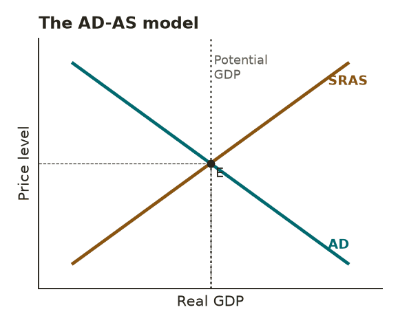
Supply and demand explain the price of gas or eggs. The AD-AS model uses the same idea for the whole economy at once. Instead of one product, the quantity is real GDP, everything the economy produces. Instead of one price, the price is the price level, an average of all prices.
OpenStax defines aggregate demand (AD) as “the amount of total spending on domestic goods and services in an economy.” That spending comes from four groups: households (consumption), businesses (investment), government (purchases), and buyers abroad (exports minus imports). These are the same four parts that add up to GDP.
The AD curve slopes down. When the overall price level rises, the money in people’s savings buys less, interest rates tend to rise, and U.S. goods become more expensive compared with foreign goods. Each of these trims the total amount people want to buy.
2 Short-run aggregate supply: total production
Aggregate supply (AS) is “the total quantity of output (i.e. real GDP) firms will produce and sell.” In the short run, the curve slopes up. OpenStax explains why: “as the price level for outputs rises, with the price of inputs remaining fixed, firms have an incentive to produce more to earn higher profits.”
The key words are “with the price of inputs remaining fixed.” Many costs are sticky in the short run. Wages are set in contracts or reviewed once a year, and rents and supply deals are signed in advance. When the prices firms can charge rise faster than their costs, producing more pays. Profits are doing what they always do: signaling where to expand. Over time, wages and other costs catch up, and that advantage fades.
3 Potential GDP: what the economy can sustain
The third piece is potential GDP, “the amount of real GDP an economy can produce by fully employing its existing levels of labor, physical capital, and technology, in the context of its existing market and legal institutions.” It is shown as a vertical line because it does not depend on the price level. It depends on workers, machines, ideas, and the rules that let people put them to use, the same forces covered in the reading on economic growth.
Where AD and short-run aggregate supply (SRAS) cross, the economy settles at an equilibrium price level and level of real GDP. That point may or may not sit at potential.
4 What shifts the curves
A change in the price level moves the economy along the curves. Other changes shift a whole curve. OpenStax sections 11.3 and 11.4 list the main causes:
| Shifts aggregate demand | Shifts short-run aggregate supply |
|---|---|
| Consumer confidence and household wealth, such as home and stock prices | Input prices, especially energy and other raw materials |
| Business confidence and investment plans | Productivity: new technology and better ways of working |
| Government spending and taxes | Wages and other labor costs |
| Interest rates, which the Federal Reserve influences | Supply disruptions: wars, pandemics, natural disasters |
| Foreign incomes and exchange rates, which change exports and imports | Business taxes and regulations that change the cost of producing |
A rightward shift is an increase, and a leftward shift is a decrease. Some events shift both curves at once, which section 8 takes up.
Measure It: Gaps and Potential
5 Recessionary and inflationary gaps
When equilibrium output is below potential GDP, the economy has a recessionary gap. Factories run below capacity and unemployment rises above its normal level. When output is above potential, the economy has an inflationary gap. Firms are stretched, workers are scarce, and wages and prices are pushed up.
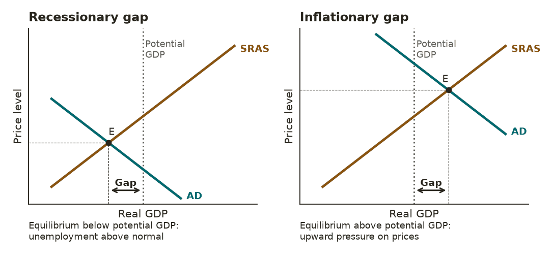
The Congressional Budget Office (CBO) estimates potential GDP, which it describes as the real GDP “that could be produced if labor and capital were employed at their maximum sustainable rates.” Comparing actual real GDP with CBO’s estimate gives the size of the gap:
| Quarter | Real GDP compared with potential | Type of gap |
|---|---|---|
| 2009, 2nd quarter | About 5% below | Recessionary |
| 2020, 2nd quarter | About 9% below | Recessionary |
| 2026, 3rd quarter | About 1.7% above | Inflationary |
By CBO’s estimates, output has been above potential since late 2021, which fits with inflation running above the Federal Reserve’s 2 percent goal. Unemployment, at 4.1 percent in October 2026, is also a bit below CBO’s estimate of its long-run normal rate, about 4.4 percent.
6 Potential is an estimate
Potential GDP cannot be observed. It has to be estimated, and the estimates change. In a well-known study, Federal Reserve economists Athanasios Orphanides and Simon van Norden found that “ex post revisions of the output gap are of the same order of magnitude as the output gap itself,” and that real-time estimates “tend to be severely biased around business cycle turning points.” So treat any gap number as a best guess, and expect it to be revised.
Explain It: Four Shocks, Four Predictions
7 What the model predicts
Shift one curve at a time, and the model makes clear predictions for real GDP, unemployment, and the price level. Dashed lines show the new curves:
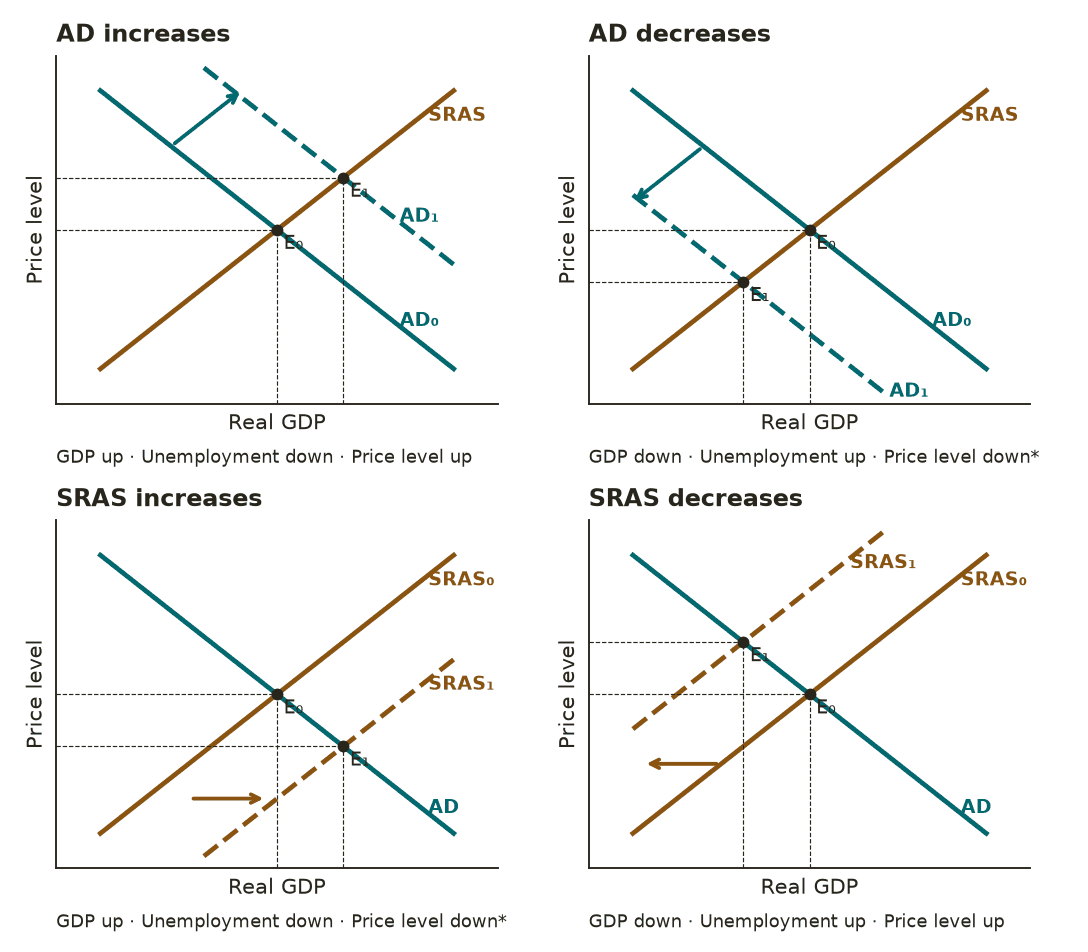
The same predictions, with the episodes from the opening:
| Shock | Real GDP | Unemployment | Price level | Example |
|---|---|---|---|---|
| AD increases | Up | Down | Up | 1965–69: war spending and new programs |
| AD decreases | Down | Up | Down* | 2008–09: housing crash and financial crisis |
| SRAS increases | Up | Down | Down* | 2014–15: oil prices fell by half |
| SRAS decreases | Down | Up | Up | 1973–75: oil embargo |
*In practice, the price level rarely falls. The model’s “down” usually shows up as slower inflation. In 2009, though, prices really did fall over a 12-month span.
WATCH The Short-Run Aggregate Supply Curve and Office Hours: Using the AD-AS Model (Marginal Revolution University)
The MRU videos put inflation and real growth on the axes instead of the price level and real GDP. The logic is the same.
8 When both curves move: the 2026 oil shock
Real events often shift more than one curve. This year is an example. After the war with Iran began on February 28, tanker traffic through the Strait of Hormuz fell from about 15 million barrels a day to 2.5 million. Brookings economists Robin Brooks and Ben Harris described the loss as roughly 20 percent of world oil supply. The price of oil rose from $72 a barrel just before the war to an average of $117 in April.
That is a textbook decrease in SRAS, and prices behaved as the model predicts. Consumer price inflation rose from 2.4 percent in January to 3.7 percent in September. Output did not. Unemployment has stayed between 4.1 and 4.4 percent all year, and real GDP grew at a 3.4 percent annual rate in the third quarter, according to a first estimate.
Why didn’t output fall? The shock starts on the supply side: higher oil prices raise costs and shift SRAS left. But when drivers and businesses pay more for oil, that money doesn’t disappear. Someone receives it. In the 1970s, much of it went to oil producers abroad, so spending in the United States fell too. Today, much of it goes to American oil producers and their workers, who spend it here.
A new study by Diego Känzig, James Stock, and Luca Zanotti shows how much that has changed. U.S. oil production rose from about 5 million barrels a day in the late 2000s to almost 14 million by 2025, and the United States became a net oil exporter in 2019. The authors find that “a rise in oil prices now boosts rather than depresses U.S. economic activity,” and that an oil shock “need no longer generate a U.S. recession.” In the model, SRAS shifts left, but AD also shifts right. The two shifts push prices up together, while their effects on output offset each other.
Drivers and airlines still pay more, so the costs fall on some people and the gains go to others. And when both curves move at once, the model can say which way prices go but not which way output goes. That depends on which shift is bigger.
9 What happens next?
The model shows where a shock moves the economy. It does not settle what happens after that. If wages and prices adjust quickly, a gap closes on its own: in a recessionary gap, costs fall and SRAS shifts back right, and in an inflationary gap, costs rise and SRAS shifts left. If wages and prices are sticky, a gap can last for years.
That question divides two broad schools of thought. Economists in the tradition of John Maynard Keynes stress sticky prices and spending, and see a larger role for policy. Neoclassical economists stress how markets adjust, and worry that policy can arrive late or add noise. The companion reading, “Should Government Fight Recessions?”, takes up that debate.
Fair Challenges
Decide what you think of each challenge first, then open the response.
“If prices are rising, the economy must be booming.”
“Falling prices are always good news.”
“High oil prices always cause a recession.”
“Low unemployment can only be good.”
Economists also disagree among themselves. Three live debates:
- What drove the 2021–22 inflation? Ben Bernanke and Olivier Blanchard concluded that “most of the inflation surge that began in 2021 was the result of shocks to prices given wages,” such as energy, food, and supply bottlenecks, and that “tight labor markets have thus far not been the primary driver of inflation.” In a new Brookings paper, Domenico Giannone and Giorgio Primiceri estimate that “approximately two-thirds of the surge in inflation after COVID was due to a boom in demand,” and note that “bottlenecks tell you where the congestion is, not necessarily what caused it.” A 2022 San Francisco Fed analysis by Adam Shapiro split the difference: supply factors explained about half of the rise, demand about a third, and the rest was unclear. In the model, this is a debate over how much AD shifted right and how much SRAS shifted left.
- How far above or below potential are we right now? CBO’s estimates put output above potential today. But because potential cannot be observed, and real-time estimates have often been revised by as much as the gap itself, some economists put less weight on gap estimates and more on what wages and prices are actually doing.
- Do recessions lower potential for good? In a 2023 review, Valerie Cerra, Antonio Fatás, and Sweta Saxena argued that deep downturns leave lasting “scars,” because lost investment and long spells out of work shrink potential. If they are right, policy should respond more actively to recessions. John Fernald, Robert Hall, James Stock, and Mark Watson studied the slow recovery after 2009 and found that slow productivity growth and falling labor force participation, trends that had begun before the recession, explained most of the shortfall. On that view, the recession itself left smaller scars.
Notice what evidence can settle and what it can’t. How much of an inflation surge came from demand, how large the output gap is, and whether recessions leave lasting damage are questions evidence can address, even when studies disagree. How to weigh lost jobs against higher prices, and who should bear the cost of a shock, are questions of values.
What Economics Adds
LISTEN What Really Drove Post-Pandemic Inflation? on the Brookings Podcast on Economic Activity, with Domenico Giannone and Giorgio Primiceri, with transcript
The Normative Question
Economics can show how demand and supply shocks move output, jobs, and prices, and why a supply shock forces a hard choice. It can’t decide which is worse: more people out of work or prices rising faster for everyone. Unemployment falls heavily on the workers who lose their jobs. Inflation is spread across everyone who buys things, and it hits hardest those whose pay does not keep up. How to weigh those costs is a judgment about values, and reasonable people weigh them differently.
Key Terms in Plain Words
- Aggregate demand (AD)
- Total spending on a country’s goods and services by households, businesses, government, and buyers abroad.
- Short-run aggregate supply (SRAS)
- The total output firms will produce at each price level while wages and other input costs are fixed.
- Potential GDP
- The real GDP an economy can sustain when it fully uses its workers, capital, and technology.
- Price level
- An average of the prices of all goods and services. Inflation is the rate at which it rises.
- Equilibrium
- The point where AD and SRAS cross, which sets real GDP and the price level.
- Demand shock
- An event that shifts AD, moving output and prices in the same direction.
- Supply shock
- An event that shifts SRAS, moving output and prices in opposite directions.
- Stagflation
- Rising unemployment and rising inflation at the same time, usually after a supply shock.
- Recessionary gap
- When real GDP is below potential and unemployment is above normal.
- Inflationary gap
- When real GDP is above potential, putting upward pressure on wages and prices.
- Output gap
- The difference between real GDP and potential GDP, as a percent of potential.
- Sticky prices and wages
- Prices and wages that adjust slowly because of contracts, menus, and habits.
Sources
- Quotations, figures, examples, and videos in this sheet come from the sources below, current as of November 6, 2026.
- The Model
- David Shapiro, Daniel MacDonald, and Steven A. Greenlaw, Principles of Macroeconomics 3e, Section 11.2, “Building a Model of Aggregate Demand and Aggregate Supply”, OpenStax, 2022 openstax.org
- David Shapiro, Daniel MacDonald, and Steven A. Greenlaw, Principles of Macroeconomics 3e, Section 11.3, “Shifts in Aggregate Supply”, OpenStax, 2022 openstax.org
- David Shapiro, Daniel MacDonald, and Steven A. Greenlaw, Principles of Macroeconomics 3e, Section 11.4, “Shifts in Aggregate Demand”, OpenStax, 2022 openstax.org
- David Shapiro, Daniel MacDonald, and Steven A. Greenlaw, Principles of Macroeconomics 3e, Section 11.5, “How the AD/AS Model Incorporates Growth, Unemployment, and Inflation”, OpenStax, 2022 openstax.org
- Marginal Revolution University, “The Aggregate Demand Curve.” youtube.com
- Marginal Revolution University, “The Short-Run Aggregate Supply Curve.” youtube.com
- Marginal Revolution University, “Office Hours: Using the AD-AS Model.” youtube.com
- The Four Episodes
- U.S. Bureau of Labor Statistics, “Unemployment Rate” (UNRATE), via FRED, Federal Reserve Bank of St. Louis fred.stlouisfed.org
- U.S. Bureau of Labor Statistics, “Consumer Price Index for All Urban Consumers: All Items in U.S. City Average” (CPIAUCSL), 12-month change calculated from seasonally adjusted data, via FRED, Federal Reserve Bank of St. Louis fred.stlouisfed.org
- Michael Bryan, “The Great Inflation,” Federal Reserve History federalreservehistory.org
- Federal Reserve History, “Oil Shock of 1973–74.” federalreservehistory.org
- Federal Reserve History, “The Great Recession.” federalreservehistory.org
- U.S. Energy Information Administration, “Crude Oil Prices Started 2015 Relatively Low, Ended the Year Lower,” Today in Energy, January 6, 2016 eia.gov
- Gaps And Potential GDP
- Congressional Budget Office, The Budget and Economic Outlook: 2026 to 2036, February 2026 cbo.gov
- Congressional Budget Office, “Real Potential Gross Domestic Product” (GDPPOT), via FRED, Federal Reserve Bank of St. Louis fred.stlouisfed.org
- U.S. Bureau of Economic Analysis, “Real Gross Domestic Product” (GDPC1), via FRED, Federal Reserve Bank of St. Louis fred.stlouisfed.org
- Athanasios Orphanides and Simon van Norden, “The Reliability of Output Gap Estimates in Real Time,” Finance and Economics Discussion Series 1999-38, Federal Reserve Board federalreserve.gov
- The 2026 Oil Shock
- Robin Brooks and Ben Harris, “The Timing of the Impending Crude Crisis,” Brookings Institution, May 22, 2026 brookings.edu
- Diego R. Känzig, James H. Stock, and Luca Zanotti, “From Importer to Exporter: Oil Shocks and the U.S. Economy,” Brookings Papers on Economic Activity, Fall 2026 conference draft, summary, September 23, 2026 brookings.edu
- U.S. Bureau of Labor Statistics, “Consumer Price Index — September 2026,” news release bls.gov
- U.S. Bureau of Economic Analysis, “Gross Domestic Product, 3rd Quarter 2026 (Advance Estimate).” bea.gov
- Debates
- Ben S. Bernanke and Olivier Blanchard, “What Caused the U.S. Pandemic-Era Inflation?” Hutchins Center Working Paper 86, Brookings Institution, June 2023 brookings.edu
- Adam Hale Shapiro, “How Much Do Supply and Demand Drive Inflation?” FRBSF Economic Letter 2022-15, Federal Reserve Bank of San Francisco, June 21, 2022 frbsf.org
- Valerie Cerra, Antonio Fatás, and Sweta C. Saxena, “Hysteresis and Business Cycles,” Journal of Economic Literature 61, no. 1 (March 2023): 181–225 aeaweb.org
- John Fernald, Robert E. Hall, James H. Stock, and Mark W. Watson, “The Disappointing Recovery of Output after 2009,” Brookings Papers on Economic Activity, Spring 2017 brookings.edu
- Podcast (With Transcript)
- Brookings Podcast on Economic Activity, “What Really Drove Post-Pandemic Inflation?” with Domenico Giannone and Giorgio Primiceri, interviewed by Louise Sheiner, November 5, 2026 brookings.edu